Matsubara Green's Function

The purpose of the second example is to treat the Matsubara Green's function by using the StochOM solver.

At first, please consider the following spectral density with two gaussian peaks:

\[A(\omega) = A_1 \exp\left[\frac{-(\omega - \epsilon_1)^2}{2 \Gamma^2_1}\right] + A_2 \exp\left[\frac{-(\omega - \epsilon_2)^2}{2 \Gamma^2_2}\right],\]

with $A_1 = 1.0$, $A_2 = 0.3$, $\epsilon_1 = 0.5$, $\epsilon_2 = -2.5$, $\Gamma_1 = 0.2$, and $\Gamma_2 = 0.8$. Then the Matsubara Green's function $G(i\omega_n)$ is evaluated by using $\mathbf{G} = \mathbf{KA}$ with $\beta = 10.0$. Random noises, built by formula $0.0001 r_1 \exp{}(i 2\pi r_2 )$ where $r_1$ and $r_2$ are random numbers in (0.0,1.0), are added to $G(i\omega_n)$. The error bar of $G(i\omega_n)$ is fixed to 1e-4. The generated data for $G(i\omega_n)$ are written in giw.data.

Next, we are going to use the standard mode, such that a configure file (ac.toml) must be prepared. It is listed as follows. Since the StochOM solver is chosen, the [BASE] and [StochOM] blocks must be present at the same time.

[BASE]
finput = "giw.data"
solver = "StochOM"
ktype  = "fermi"
mtype  = "flat"
grid   = "ffreq"
mesh   = "linear"
ngrid  = 10
nmesh  = 501
wmax   = 5.0
wmin   = -5.0
beta   = 10.0
offdiag = false

[StochOM]
ntry  = 100000
nstep = 1000
nbox  = 100
sbox  = 0.005
wbox  = 0.02
norm  = -1.0

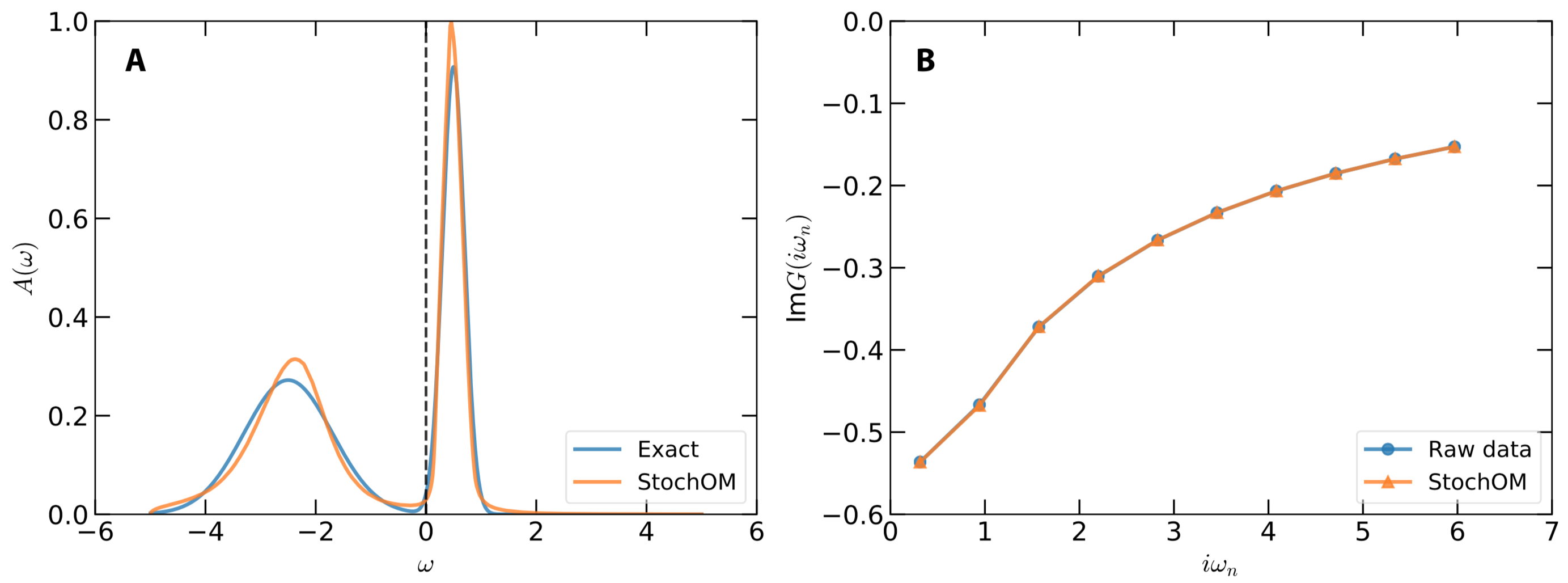
Then we use the acrun.jl or Pacrun.jl script to perform analytic continuation simulation. The calculated results are shown in Fig.1. As is seen in Fig.1(a), both the sharp peak around 0.5 eV and the broad peak around -2.5 eV are correctly reproduced by the StochOM solver. In Fig.1(b), the reconstructed Matsubara Green's function agrees quite well with the raw input data.

Figure 1 | Analytic continuation of Matsubara Green's function by using the stochastic optimization method. (a) Simulated and exact spectral functions. (b) Reconstructed and synthetic Matsubara Green's functions. Only the imaginary parts are presented in this figure.