General Coulomb interaction

Introduction

In this tutorial, we will show you how to use the iQIST software package to solve a two-band Hubbard with rotationally invariant Coulomb interaction.

The interaction term of the Hubbard model are as follows:

\[\begin{align} \hat{H}_{\text{loc}} = &- \mu \sum_{\alpha\sigma}n_{\alpha\sigma} + U\sum_{\alpha} n_{\alpha\uparrow}n_{\alpha\downarrow} \\ & + U^{\prime} \sum_{\alpha > \gamma, \sigma} n_{\alpha\sigma}n_{\gamma\bar{\sigma}} + (U^{\prime} - J) \sum_{\alpha > \gamma, \sigma} n_{\alpha\sigma}n_{\gamma\sigma} \\ & - J \sum_{\alpha \neq \gamma} (d^{\dagger}_{\alpha\downarrow}d^{\dagger}_{\gamma\uparrow}d_{\gamma\downarrow}d_{\alpha\uparrow} + d^{\dagger}_{\gamma\uparrow}d^{\dagger}_{\gamma\downarrow}d_{\alpha\uparrow}d_{\alpha\downarrow} + h.c.). \end{align}\]

Here $\alpha$ and $\gamma$ are the orbital indices, $\sigma$ the spin index, $\mu$ the chemical potential, $U$ ($U^{\prime}$) the intra-orbital (inter-orbital) Coulomb interaction, and $J$ the Hund's exchange interaction. Unless otherwise specified, $\mu$ is chosen to meet the half-filling condition. The $U$ ($U^{\prime}$) and $J$ parameters fulfill the relation $U^{\prime} = U - 2J$. In this tutorial, a semicircular density of states with half bandwidth $D = 2t$ is used, which corresponds to the infinite-dimensional Bethe lattice. We solve the Hubbard model using single-site DMFT with a state-of-the-art CT-HYB quantum Monte Carlo impurity solver.

The model parameters are as follows:

• $U_c$ = 4.0
• $U_v$ = 2.0
• $J_z$ = 1.0
• $J_s$ = 1.0
• $J_p$ = 1.0
• $\mu$ = 3.50

Recipes

Next we just follow the procedures described in the iQIST recipes section.

(1) Choose suitable component

Since the local Hamiltonian contain the spin-flip and pair-hopping terms, it is not diagonal under the occupation number basis. So the segment representation algorithm is not valid in this case. We have to use the general matrix version of CT-HYB quantum impurity solvers. In this tutorial, we choose the BEGONIA component to solve it. Of course, the LAVENDER, PANSY, MANJUSHAKA, and CAMELLIA components are also applicable.

(2) Design the programs and scripts

Since the Hubbard model is defined in a Bethe lattice whose density of states is semi-circular, the self-consistent equation for the dynamical mean-field theory reads:

\[G(\tau) = t^2 \Delta(\tau)\]

As mentioned before, the BEGONIA component (and the other quantum impurity solver components) contains a mini dynamical mean-field engine and the above self-consistent equation is already implemented by default. So, we can use the BEGONIA component alone without help from any external programs or scripts.

(3) Prepare the input files

Please create a working directory for this tutorial:

$ mkdir test21

As for the BEGONIA component (and the other general matrix version of CT-HYB quantum impurity solvers), the atom.cix file is always necessary. Without it, the impurity solver won't run correctly. We have to use the JASMINE component to generate it at first. The configuration file (atom.config.in) for the JASMINE component is attached as follows:

!!!-----------------------------------------------------------------------
!!! source  : t21/atom.config.in
!!! solver  : JASMINE
!!! purpose : for tutorial
!!! author  : yilin wang (email:qhwyl2006@126.com)
!!!-----------------------------------------------------------------------

!!>>> setup general control flags
!!------------------------------------------------------------------------
  ibasis : 1
  ictqmc : 1
  icu    : 1
  icf    : 0
  isoc   : 0

!!>>> setup common variables for jasmine
!!------------------------------------------------------------------------
  nband  : 2
  nspin  : 2
  norbs  : 4
  ncfgs  : 16
  nmini  : 0
  nmaxi  : 4

!!>>> setup common variables for jasmine
!!------------------------------------------------------------------------
  Uc     : 4.00
  Uv     : 2.00
  Jz     : 1.00
  Js     : 1.00
  Jp     : 1.00
  Ud     : 0.00
  Jh     : 0.00
  lambda : 0.00
  mune   : 0.00

Please setup your atom.config.in file, or just copy it from the iqist/tutor/t21 directory:

$ cp iqist/tutor/t21/atom.config.in test21

In the atom.config.in file, the local Hamiltonian is defined. Then we solve it using the JASMINE component.

$ cd test21
$ pwd
$ atomic

Here atomic is the executable program of the JASMINE component. We assume that it is in the iqist/build directory and added to the PATH. The atomic is extremely fast. After the calculation is finished, there are a lot of output files in the test21 folder. Try to find out the atom.cix file and ignore the others. Is it ready? You can use any text editor to open and read the atom.cix file. But please don't edit it for ever.

Next we have to prepare the solver.ctqmc.in file for the BEGONIA component. An official version is attached as follows.

!!!-----------------------------------------------------------------------
!!! source  : t21/solver.ctqmc.in
!!! solver  : BEGONIA
!!! purpose : for tutorial
!!! author  : yilin wang (email:qhwyl2006@126.com)
!!!-----------------------------------------------------------------------

!!>>> setup general control flags
!!------------------------------------------------------------------------
  isscf  : 2
  issun  : 2
  isspn  : 1
  isbin  : 1

!!>>> setup common variables for quantum impurity model
!!------------------------------------------------------------------------
  nband  : 2
  nspin  : 2
  norbs  : 4
  ncfgs  : 16
  nzero  : 256
  niter  : 20
  U      : 4.00
  Uc     : 4.00
  Uv     : 2.00
  Jz     : 1.00
  Js     : 1.00
  Jp     : 1.00
  mune   : 3.50
  beta   : 10.0
  part   : 0.50
  alpha  : 0.70

!!>>> setup common variables for quantum impurity solver
!!------------------------------------------------------------------------
  mkink  : 1024
  mfreq  : 8193
  nfreq  : 128
  ntime  : 1024
  npart  : 4
  nflip  : 20000
  ntherm : 20000000
  nsweep : 200000000
  nwrite : 20000000
  nclean : 100000
  nmonte : 100
  ncarlo : 100

But you can also copy it from the iqist/tutor/t21 directory:

$ cp iqist/tutor/t21/solver.ctqmc.in .

The important parameters in the solver.ctqmc.in file are as follows:

• isscf = 2: Define the DMFT self-consistent computational mode.
• nband = 2, norbs = 4, and ncfgs = 16: Specify a two-band Hubbard model.
• nzero = 256: Maximum number of non-zero matrix elements for F-matrix.
• mune = 3.5 : Chemical potential $\mu$.
• beta = 10.0 : Inverse temperature $\beta$.
• npart = 4: Number of parts that the imaginary-time axis is splitted.

In fact, you can create a simplified solver.ctqmc.in file which contains only the nband, norbs, ncfgs, nzero, mune, and beta parameters. The BEGONIA component will supplement the rest using default settings. Noted that now the Uc, Uv, Jz, Js and Jp parameters in the solver.ctqmc.in file are used as a reference. All of the information about the local Hamiltonian is defined in the atom.config.in file and dealed with the JASMINE component. The BEGONIA component is not responsible for constructing the local Hamiltonian model.

As for the format and grammar for the solver.ctqmc.in file, see solver.ctqmc.in for more details.

(4) Let's go

Now everything is ready. We can perform the calculation. Please execute the following command in the terminal, and then do another job. This calculation will cost you about five hours.

$ ctqmc

(5) Post-processing

As usual we use the Python/matplotlib package to visualize the calculated results. If you are not familiar with this powerful tool, please visit its official website:http://matplotlib.org. Here is a sample Python script for plotting the imaginary-time Green's function $G(\tau)$, you can modify it to fit your requirements.

#!/usr/bin/env python

import numpy
import matplotlib
matplotlib.use("Agg") # setup backend
import matplotlib.pyplot as plt

# read data
beta = 10.0
bi, ti, tau, gtau, error = numpy.loadtxt('solver.green.dat', unpack = True)
tau = tau[0:1023] / beta

# plot it
plt.figure(0)
lines = plt.plot(tau, gtau[0:1023], alpha = 0.8, clip_on = True)

# setup line properties
plt.setp(lines[0], linewidth = 2.5, color = 'khaki')

# setup tics
plt.xticks(fontsize = 18)
plt.yticks(fontsize = 18)
plt.tick_params(length = 8, width = 1.0, which = 'major')
plt.tick_params(length = 4, width = 0.5, which = 'minor')

# setup labels
plt.xlabel(r"$\tau/\beta$", fontsize = 18)
plt.ylabel(r"$G(\tau)$", fontsize = 18)

# setup yranges
plt.xlim(0.0,1.0)

# output the figure
plt.savefig("21gtau.png")

Next we will show some visualized results. The following figures were generated using the above Python script with slight modifications. You can compare them with your own results to see whether your calculations are correct.

• Histogram (solver.hist.dat)

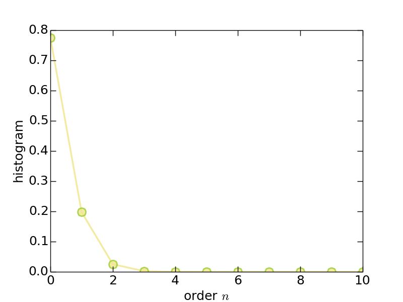
Figure | The histogram for perturbation expansion series.

• Imaginary-time Green's function (solver.green.dat)

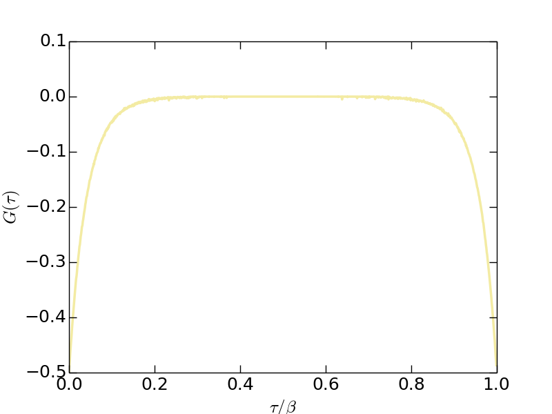
Figure | The imaginary-time Green's function $G(\tau)$.

• Matsubara Green's function (solver.grn.dat)

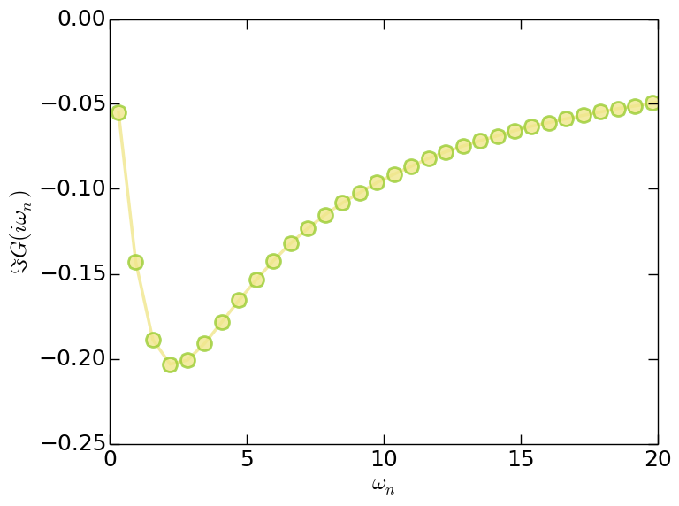
Figure | The imaginary part of Matsubara Green's function $\Im G(i\omega_n)$.

• Matsubara self-energy function (solver.sgm.dat)

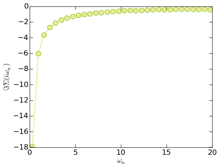
Figure | The imaginary part of Matsubara self-energy function $\Im \Sigma(i\omega_n)$.

Since the orbitals in this model are degenerated, so for $G(\tau)$, $G(i\omega_n)$, and $\Sigma(i\omega_n)$ we only plot the data for the first band. Clearly, the system is in insulating state.

Adventures

(1) Adjust the parameters

You can adjust the mune, beta, npart, and nsweep parameters, and redo the calculations, to see what will happen.

(2) Parallel computation

Try to execute the CT-HYB quantum impurity solvers parallelly. Such as

$ mpiexec -n 8 ctqmc

This will greatly reduce the numerical fluctuation in physical observable with the same nsweep parameter.

(3) Try the LAVENDER component

Use the LAVENDER component to do the calculation again. The original atom.cix file can be used directly. The solver.ctqmc.in file can be the same.

(4) Try the PANSY and MANJUSHAKA components

Since the atom.cix used by the BEGONIA and LAVENDER components is not compatible with the one used by the PANSY and MANJUSHAKA components. So we have to rebuild the atom.cix file at first. Please change ictqmc from 1 to 2 in the atom.config.in file, and then use the JASMINE component to generate the atom.cix file again. Then you can execute the PANSY or MANJUSHAKA component to solve the model. It is unnecessary to modify the solver.ctqmc.in file. Finally, you can compare the calculated results obtained by these two kinds of general matrix version of CT-HYB quantum impurity solvers. That's all.